CFD & Structural Analysis of ONERA M6 Wing
Calibrated ONERA M6 wing transonic aerodynamics against NASA data, achieving 4.9% and 11.2% error for lift and drag, and evaluated stress and deformation using a one-way Ansys Fluent to Mechanical pipeline. I took this on as a personal interested project to expose myself to Ansys Fluent and investigate how CFD data can be used to inform structural loading cases.
The ONERA M6 wing is a classic transonic validation case for CFD models. At high Mach numbers, regions of subsonic and supersonic flow develop, and turbulent boundary layer separation occurs [1]. This in turn contributes to increased drag and the potential for shock waves, making it an interesting case for hyper speed aviation.
The M6 wing was tested based on the conditions published in Test 2308:

To evaluate the flow behavior, a Spalart-Allmaras turbulence model is used in Ansys Fluent and evaluated against the results on NASA’s website. Both the lift and drag showed good alignment with NASA’s highest resolution results, with a 4.9% underestimation of the lift coefficient and 11.2% overestimation of the drag coefficient [2]. Improved accuracy could be achieved through a greater refinement in the mesh and reducing the residuals. However, these approaches have greater computational cost and longer run times, a common limitation for student based computational resources.
The Wing
The geometry is based on ONERA’s M6 wing, characterized by the following parameters [3], [4]:


CFD Model
Source: [5]
A Spalart-Allmaras turbulence model is used to track the turbulence within the flow field [6]. Solving the standard Spalart-Allmaras model can introduce small negative turbulence values which cause solution instability [7]. However, instead of clipping these values, a revised conditional form of the model is used to directly address the negative values. An extensive break down of this model is highlighted here.
Using the provided testing configuration data from Test 2308, the properties of the flow can be found. The free stream velocity (u∞) is based on the Mach number (M) and the speed of sound in air (c).
Where, the speed of sound it air is dependent on the temperature (T), ratio of specific heat (γ) and specific gas constant for air (R) [8].
The free stream density (ρ∞) can be found by rearranging a standard form for the Reynold’s number. For this case, the characteristic length is assumed to be the wing’s root chord.

Sutherland’s Law is used to describe the temperature dependence of the dynamic viscosity (μ), with respect to the reference temperature (Tref) and Sutherland constant (S) [9].

The flow properties used in model are shown below.

Boundary Conditions
Farfield conditions are used at the hemispherical boundaries, with pressure (98178.31 Pa) described by the ideal gas law:
and the turbulent viscosity (4.8574e-05 m^2/s) assumed to take the form below.

Mesh
To develop a quality mesh, the element sizing closest to the airfoil surface must be small enough to capable to capture flow behavior due to friction along the fluid-solid interface. Determining the appropriate local element size (Δs) can be done using a wall-resolved mesh sizing approach.

The friction velocity (ufric) is defined below.


Where τwall is the wall shear stress and Cf is the coefficient of skin friction, and y+ is a non-dimensional variable used to describe where the first element is located within the sublayers of the boundary flow. When y+ < 1, the first element is within the viscous sublayer, while 5 < y+ < 30 means that the first element is in the buffer layer [10]. For this simulation, a y+ value of 20 was used due to limited computational resources. This sacrifices the ability for the model to accurately capture the flow behavior close to the wing but provides reasonable approximations for the lift and drag coefficients.
Results
The lift and drag coefficients were found to be 0.2561 and 0.0189 respectively. The error in these values with respect to NASA data (4.9% and 11.2%) directly reflects a low level of mesh refinement, which was restricted due to limited computational resources. Larger element sizes struggle to capture the steep pressure gradients, suppressing suction peaks leading to underestimation of lift. Similarly, element size effects the velocity gradient at the boundary which can artificially increase the calculated viscous forces and overestimate drag.
The effects of element size on the lift and drag coefficients are further highlighted by NASA data in the plots below. The low mesh resolution shows lift coefficients as low as 0.2562, only 0.03% different from the results found using Ansys Fluent. NASA’s drag coefficient is shown to be as great as 0.0230, with finer resolution meshes converging to a drag coefficient of 0.0170. This suggests that the Ansys Fluent results are within an acceptable range. For greater accuracy, future simulations should use a y+ value of less than 1 to provide better representation of the boundary layer behavior and improve the pressure and velocity fields.


To analyze alignment of the pressure field with NASA data, plots were generated for the coefficient of pressure for cross sections located at 20%, 65%, 80% and 99% of total wing length. Following aerodynamic convention, the y-axis is inverted so that suction plots upwards and the top surface is represented by the top curve. The plots show that the Ansys Fluent results underpredict suction, with an earlier decay in the shock wave, a consequence of poor boundary layer representation due to larger element sizing.

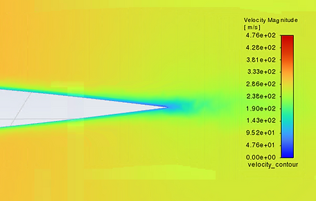
Additional pressure and velocity cross section profiles from the base of the wing are shown below. The pressure on the wing surface in the bottom right contour plot will be used in a structural load simulation to understand how the aerodynamic induced forces contribute to stress distributions within the wing.


Structural Response
A one-way pipeline was created from Ansys Fluent to Mechanical to evaluate the structural response of the wing. Using the pressure field data, a distributed load was applied to the wing surface, while the base of the wing was held fixed. The goal of this study is to highlight multi-physics FEA, where CFD creates informed loading for structural models. Since documentation on the interior geometry of the ONERA M6 wing is limited, I generated a generalized form where the interior of the wing is hollow, with a wall thickness of 6.35 mm, and the trailing edge was reinforced with a wedge of extra material to prevent an unrealistic sharp interior edge. While this geometry does not directly reflect standard wing design, it does provide a platform for analyzing the effects of the fluid-based loading.

One of the challenges of meshing a design of this nature is the thickness to length ratio. Thin features that undergo bending must be represented by multiple elements through their thickness. As a result, decreasing the wall thickness rapidly drives up the total element count. Additionally, limited access to computational resources reduces the ability to develop fine meshes, therefore, it was not possible to consider significantly thinner walls.
von-Mises Stress
The von-Mises stress contour plots reflect the effects of cantilever bending from the lift force, and the pressure jump caused by the transonic shock. The maximum von-Mises stress (61.23 MPa) occurs at the root in the thin wall region, where the bending moment is the greatest and shell is most compliant.
By fixing the root, material deformation along the boundary is constrained, introducing high shear stress in adjacent elements and an artificial magnitude for the local stress peak. Analysis of the von-Mises stress contour should therefore not consider stress values closest to the root as they poorly reflect material behavior.
Additionally, the transition between the trailing wedge and the thin wall introduces a stress concentration caused by a reduction in the effective load carrying area. Increasing the size of fillets along this transition would reduce the stress concentrations.
.png)
Vertical Deflection
The lift force causes the wing to bend upwards with the highest vertical deflection (2.04 mm) occurring at the tip. Compared to the wing length of 1.196 m, the magnitude of the deflection is minimal, having limited impact on the effective geometry. This suggests that a one-way pipeline may be appropriate for evaluating the static case.

References
[1] T. Takahashi, Aircraft performance and sizing. Volume I : fundamentals of aircraft performance. in Aerospace engineering collection. New York, NY: Momentum Press, 2018.
[2] C. Pederson, “Turbulence Model Numerical Analysis 3D ONERA M6 Wing Validation,” Turbulence Modeling Resource. [Online]. Available: https://turbmodels.larc.nasa.gov/onerawingnumerics_val_sa.html
[3] C. Pederson, “Turbulence Model Numerical Analysis 3D ONERA M6 Wing Validation,” Turbulence Modeling Resource. [Online]. Available: https://turbmodels.larc.nasa.gov/onerawingnumerics_val.html
[4] V. Gleize, A. Dumont, J. Mayeur, and D. Destarac, “RANS simulations on TMR test cases and M6 wing with the Onera elsA flow solver,” in Turbulent Flow Solutions for NACA 0012 and Other Test Cases from the Turbulence Model Resource Website: Residual and Grid Convergence II, Kissimmee, Florida, Jan. 2015. doi: 10.2514/6.2015-1745.
[5] S. Gaultier, “ONERA-M6 Wing, Star of CFD,” ONERA. Accessed: Aug. 25, 2025. [Online]. Available: https://www.onera.fr/en/news/onera-m6-wing-star-of-cfd
[6] P. R. Spalart and C. L. Rumsey, “Effective Inflow Conditions for Turbulence Models in Aerodynamic Calculations,” AIAAJ, vol. 45, no. 10, pp. 2544–2553, Oct. 2007, doi: 10.2514/1.29373.
[7] “The Spalart-Allmaras Turbulence Model,” NASA Langley Research Center Turbulence Modeling Resource. Accessed: Aug. 20, 2025. [Online]. Available: https://turbmodels.larc.nasa.gov/spalart.html
[8] T. Benson, “Speed of Sound,” Glenn Research Center (NASA). Accessed: Aug. 26, 2025. [Online]. Available: https://www.grc.nasa.gov/www/k-12/VirtualAero/BottleRocket/airplane/sound.html
[9] “Sutherland’s law,” CFD Online. Accessed: Aug. 28, 2025. [Online]. Available: https://www.cfd-online.com/Wiki/Sutherland%27s_law
[10] “What Is y+ In CFD? – And Why Does It Matter?,” Fidelis. Accessed: Aug. 28, 2025. [Online]. Available: https://www.fidelisfea.com/post/what-is-y-in-cfd-and-why-does-it-matter