Vehicle Dynamics Modeling

Ride comfort and handling are two critical considerations in vehicle design. Suspension design, tires and weight distribution play a major role in defining how a vehicle responds to both road and driver inputs. I explored transient vehicle models to study the dependence of ride and handling performance on design parameters, inform vehicle optimization, and assess stability and natural frequencies.

The behavior of a vehicle on a roadway can be characterized by vehicle dynamics models, which capture the response of a vehicle to road and steering inputs. Changes in the road topography and the driver’s steering maneuvers will cause mechanical interactions between the road, tires, wheel uprights, steering mechanism, suspension system, and the chassis of the vehicle. Each of these interactions plays a critical role in characterizing a vehicle’s overall ride and handling performance.

To track the dynamic behavior of the vehicle, a coordinate system must be assigned to the vehicle. The diagram below details the standard coordinate system orientation used in the models contained in this report. Here the downwards is the +Z direction, the +Y direction is towards the right side, and +X is in the direction that the vehicle is facing. Rotations about this coordinate system are denoted as the yaw angle (ψ), pitch angle (θ), and the roll angle (φ). These angles are critical for identifying weight transfer in the lateral and longitudinal directions, as well as the changes in the direction of vehicle heading.

Suspension design plays a critical role in ride and handling of a vehicle, with the ability to tune the response of the system to address different road and steering inputs. Below are a few different models that are commonly used to understand the response modes associated with passenger vehicles. Click on the tabs to get a breakdown of each model.

Ride Models

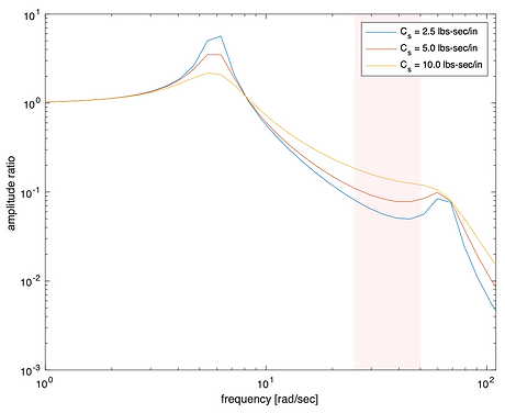
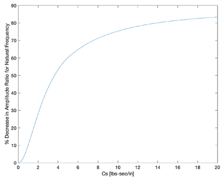
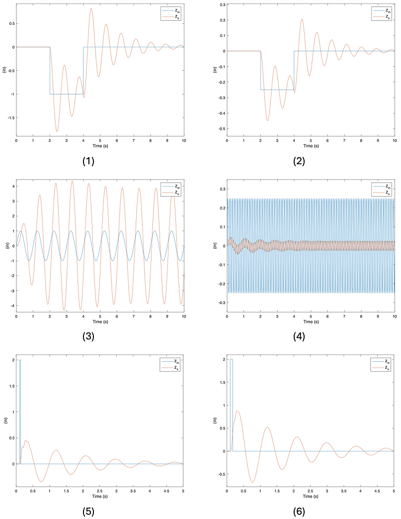
The ride characteristics of a consumer vehicle strongly influence the passenger experience. A vehicle can be represented by a system of springs, dampers and masses, to better understand the associated natural frequencies and transient responses to different road inputs. Experimental studies have shown that frequencies between 4 to 8 Hz can create the greatest discomfort for drivers and passengers, making it critical to identify the road-induced frequencies within this range that could excite the suspension system [1]. Two different ride models, a quarter car model, and a pitch-plane model are used to analyze the vehicle responses to vertical road inputs. The quarter car model analyzes the motion of a single wheel, representing a quarter of the full vehicle system, while accounting for a quarter of the sprung mass (chassis and body weight) and the unsprung mass (wheel assembly). The pitch-plane model captures the heave and pitch motion responses of the vehicle by considering the front and rear suspension assemblies along with key chassis parameters including sprung mass, the location of the center of gravity, and pitch moment of inertia. This model can also be extended to a half car model that includes the tire stiffness and damping, suspension damping, and the unsprung masses (front and rear axle weights).

The quarter car model is an idealized two-mass system that allows for an approximated dynamic response of a vehicle suspension to heave based inputs. In the system, the sprung mass (chassis/body) is connected to the unsprung mass (wheel hub assembly) by a spring and damper. The hub is then “connected” to the ground by the tire which can be represented by another spring and damper.

In this assembly, the downwards direction is the +z direction, where z_s, is the displacement of the sprung mass, z_u is the displacement of the unsprung mass, and z_in is the displacement of the ground. The spring stiffnesses, K_s and K_t, are the suspension and tire stiffnesses respectively, and Cs and Ct are the damping coefficients for the suspension and tire. The masses, m_s and m_u, are the sprung and unsprung masses. For the linear model, the following values will be used:

For this model, the following values are used:

** This parameter is to be varied.

Dynamics

The quarter car model can be described in both the time domain (state-space) or the Laplace s-domain. While the s-domain can be useful for analyzing the system and allow for the use of Simulink, it is more difficult to use in cases where non-linear damping is used. Therefore, both versions of the model are developed below.

State-Space

The forces within the system are described by the equations below.

The system can then be rearranged and presented in a state-space form.

Laplace s-domain

Using Laplace transform, Equation 1 and 2 can be rewritten to be expressed in terms of s.

This can be expressed in matrix form:

Natural Frequencies

The natural frequencies of the quarter car model can be analyzed to determine how changes in stiffness and damping affect the driver comfort. Human sensitivity to vibrations has been shown to be the highest in the frequency band of 4-8 Hz. Therefore, it is important to analyze the suspension damping and stiffness parameters to minimize frequencies in this range while maintaining low amplitudes for natural frequencies. Using the state-space model, the parameters in the table above and Cs = 5 lbs*sec/in, the following plot was generated using a Bode plot function in Matlab to determine the amplitude ratio associated with a given frequency.

In the left plot, the first large peak is the natural frequency associated with the sprung mass, while the second large peak is the natural frequency for the unsprung mass (wheel hop). In the right plot, increasing the suspension damping coefficient decreases the amplitude ratio for the sprung mass natural frequency, however this comes at the tradeoff of increased amplitude for frequencies within the sensitivity band. The goal is to minimize natural frequency amplitude ratio and minimize the amplitude ratios of frequencies within the sensitivity band.

To calculate the performance effects of increasing the damping coefficient, amplitude ratios of the damped configuration were calculated as functions of damping coefficient, and then compared to amplitude ratios of the undamped configuration.

By tracking the percent change in the amplitude ratios, the return on increased damping can be quantified.

(Left plot)

For the amplitude ratio of the sprung mass natural frequency, the percent improvement is greater at small values of Cs, but returns begin to quickly decline as Cs gets large. The rate of increase in the maximum amplitude ratios within the sensitivity band is shown to be smaller at Cs = 4 lbs-sec/in, but has a steeper linear percent change for greater Cs values.

(Right plot)

To choose an optimal Cs for this analysis, the percent changes in amplitude ratios were compared. At the chosen value, Cs = 4 lbs-sec/in, there is a 43% increase in the maximum amplitude ratio experienced in the sensitivity band, but a 53% decrease in the amplitude ratio for the sprung mass natural frequency. This point marks the start of reduced performance returns based on the above plots.

In the future, stronger optimization and weighting functions should be used to make more informed decisions, however, this general approach provides a starting point for the analysis.

Simulating Responses to Road Inputs

There are six different input cases for that will be considered:

A 1-inch step function at 0.5 Hz
A ¼ inch step function at 0.5 Hz
A +/- 1-inch sine wave input at 1 Hz
A +/- ¼ inch sine wave at 10 Hz
A 2-inch pothole 3 ft wide at 60 mph
A 2-inch pothole 3 ft wide at 30 mph

These input cases are shown in the figures below.

Using the linear damping model and the Cs value (4 lbs-sec/in) found in the previous section, the system was tested using the input functions to better understand the response to different types of road inputs.

A couple key observations include high overshoot for step functions with a longer period, high amplitude ratios for the 1 Hz wave, and undershoot for the step functions with short periods that are less than the system rise time. The high overshoot and longer settling times suggests that further tuning should be conducted to find a more appropriate damping parameter. In addition, the introduction of non-linear damping and rebound rate control are potential ways to optimize system response.

The pitch plane model is an idealized system that approximates the dynamic heave and pitch response of vehicle suspension based on vertical displacement inputs at the front and rear axles. In the system, the sprung mass (chassis/body) is connected to the front and rear axles by springs. In this model variation, the unsprung masses are not considered, and the shock and tire stiffnesses are represented by an equivalent stiffness.

The pitch-plane model captures vertical displacement and pitch rotation of the vehicle body based on front and rear suspension forces and assumes small angle approximations.

The state-space model can then be expressed as:

The pitch-plane model captures vertical displacement and pitch rotation of the vehicle body based on front and rear suspension forces and assumes small angle approximations.

Natural Frequencies

To determine the natural frequencies of the pitch-plane model, the state-space equations are transformed into the frequency domain using the Laplace transform and solved via the characteristic equation. Further simplifying relations are used:

The resulting heave and pitch natural frequencies are:

Olley Ride Criteria

The Olley Ride Criteria is a method used to optimize the ride quality of a consumer vehicle with regards to its pitch-plane behavior. These three criteria improve ride comfort by addressing a vehicle’s suspension frequency response.

The heave and pitch natural frequencies should be less than 1.3 Hz to ensure passenger comfort.
The heave frequency should be less than 1.2× the pitch frequency.
Deflection of the front suspension should be at least 30% greater than the rear to reduce pitch acceleration (i.e., spring center forward of CG).

These targets guide the choice of front and rear stiffnesses during vehicle design and tuning.

System Testing Results

There are six different input cases for that will be considered:

A 1-inch step function at 0.5 Hz
A ¼ inch step function at 0.5 Hz
A +/- 1-inch sine wave input at 1 Hz
A +/- ¼ inch sine wave at 10 Hz
A 2-inch pothole 3 ft wide at 60 mph
A 2-inch pothole 3 ft wide at 30 mph

Both the front and rear axles will be subjected to the same inputs; however, the vehicle wheelbase length must be accounted for by introducing a speed dependent time delay for the rear axle input relative to the front axle.

The half car model builds on the pitch plane model by including the unsprung masses of both front and rear axles, suspension dampers, and the tire stiffness and damping.

The forces within the dynamic system are described by:

The positions z_1 and z_2 can be written in terms of z_s and θ.

Under the assumption of small angle approximation, sinθ≈θ and cosθ≈1. Additionally, the relationships between the spring stiffnesses and dampers can be simplified.

The state-space model can then be expressed as:

Using an Explicit Euler Method with the state-space form can be used to solve for the time evolution of the system over a small-time increment.

Transient System Response

The results of the system will be uploaded shortly.

Handling Models

Vehicle handling characteristics play a critical role in a driver’s control over the vehicle. When a driver provides a steering input through the handwheel (steering wheel), the direction that the tires are pointing differs from the vehicle heading, introducing a tire slip angle. The resulting tire deformation generates lateral cornering forces at the tire contact patches. This occurs at both the front and rear tires, contributing to a net yaw moment that influences the vehicles direction of heading. The yaw rate model is built upon the classic bicycle model force diagram to capture the yaw rate and drift angle response of a vehicle during a handling maneuver. The model accounts for the yaw moment of inertia, wheelbase, center of mass, vehicle mass, and cornering stiffness of the tires. This model was extended to include roll dynamics, incorporating the roll moment of inertia, roll stiffness, roll damping, and non-linear tire behavior that arise from weight transfer across an axle. Lastly, a simplified steering compliance model was developed to examine how resisting moments at the tire contact patches, torsional compliance of the steering column, and steering system geometry affect the vehicle response to a handwheel input.